You Could Have Come Up with Speculative Decoding
Building up speculative decoding from first principles
Speculative Decoding is a great example of how good systems understanding can lead to performance increases; in some case around decode throughput.1 It is kind of a perfect study since it involves knowing the entire inference stack from batch scheduling, hardware limitations to the model internals to make it work well.
Starting with the Constraints#
Lets dive into how you could have also come up Speculative Decoding. Whenever you think of optimization, you might imagine various axes of freedom the problem has e.g. to get a specific result you might be able to add more compute, this is a variable you could change; although the relation might not be linear, but the idea is there is a relation. Start with the boundary conditions for our problem; first, you might know that autoregressive decoding is
-
Memory-bound, you can’t just add more compute and expect better results2 for small number of batches and
-
you have to generate the -th token before you can generate the -th token, meaning decode is inherently sequential.
Note that boundary conditions are just arbitrary here, they are soft conditions to simplify the systems model3. Here is what I think our axes might be.
-
You could find a way to reduce what is loaded from memory, you would stop being memory limited and get closer to the memory/compute roofline. This is where ideas around various attention variants (MQA, GQA etc.) and KV compression techniques lie.4
-
Use more of the compute available, since anyways the model needs to be loaded from memory, might as well do more compute for that load.
-
Batch scheduling; when serving a model to a lot of users, you can schedule a number of these decode requests together to a) amortize the cost of loading the full model across all the requests5 and b) more efficiently use more of the available compute.
In some techniques, the axes might be coupled e.g. with quantization you get a better FLOPs/bytes both due to higher FLOPS being possible on low bit data types and reduced memory movement due to small size.
Not Every Token is Equal#
Another observation about natural language; which I think almost everybody would know intuitively; is that language has a lot of redundancies and easy repeatable patterns around grammar, repeated phrases and writing conventions.6 And you are spending full model’s worth compute and memory to predict something that might locally be very easy to predict, lets take a side quest first to understand this more.
At each decode step, the model has a next token distribution sample from
Here Information Theory gives a way to quantify how predictable this next token is. For the realized token , define its information content (or surprisal), under the model as
Higher the probability, lesser the new information the token carries and vice versa. Here is a heatmap visualization of how the information content varies with as the sentence becomes syntactically richer.
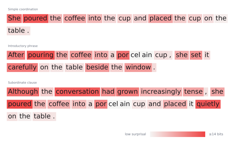
Observed-token information content across three variations of the same scene, measured locally with GPT-2 Large (774M parameters). Brighter red means the observed token received less probability from the model. Blocks follow the model’s tokenization, so a word can span several blocks.
But the amount of information is know only after a token is sampled from the distribution. To gauge the a sense of the next token information without selecting a token, you would think about aggregate metrics like what would be the expected information value under . This is the conditional entropy of the token
Entropy therefore measures how uncertian is the model about its own outcomes. An entropy of bits corresponds very loosely to a choice among equally likely choices. Although the full vocabulary may have a lot many tokens, at many positions grammar, repitition, formatting and semantic context reduces a lot choices.
Guessing is Enough?#
This observation suggests another systems opportunity. If a lot of next-token distributions have low entropy, perhaps you don’t need the full large model to predict every token. Remember that decode is memory-bound and has some unused compute capacity.
A cheap proposal mechanism could predict the easy patterns in natural language and manufacture a provisional block of future tokens, . It could be a smaller autoregressive model, a parallel prediction model, an n-gram lookup, or a continuation copied from the existing context. Its purpose is to provide the future tokens needed to expose parallel work for the large model. For example, say “The cat” is and the proposed next tokens are “sat on a mat” (s).
Now these proposals might be totally wrong. How do you verify them cheaply? First, simply run a causally masked forward pass on the sequence and get distributions from the large model conditioned on the preceding draft prefix. These are calculated at a better arithmetic intensity than vanilla decode. Assuming you are using greedy decoding7, you would get
What do you do with these? Notice how you can verify the entire sequence using this forward pass by comparing s and s. If they match the draft prediction, keep the token; at the first mismatch, emit the large model’s token and drop the remaining draft tokens. The expectation is that more often than not a good chunk of the draft sequence will match. In the example above, say verification gives “sat”, “on”, “the” while the draft proposed “sat on a mat”. The first two tokens match and are kept, “the” is emitted from the large model, and “a mat” is dropped because it was conditioned on a token that was not accepted.
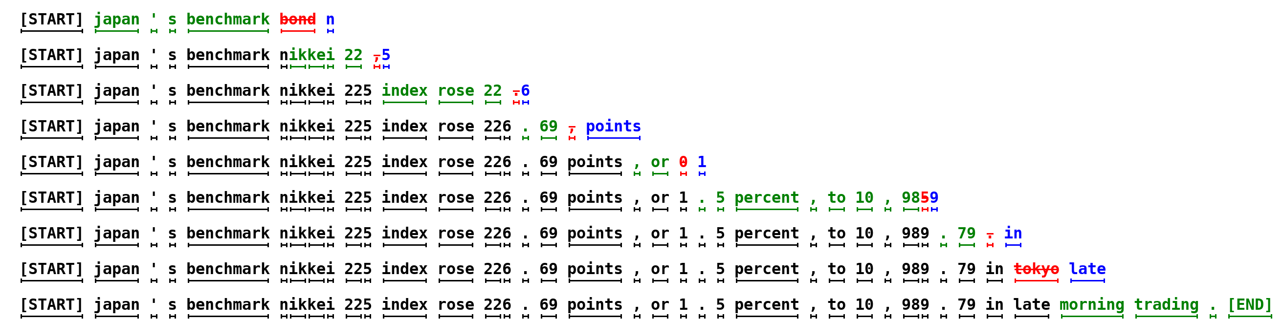
A complete decode trace from Figure 1 of Leviathan et. al.. Each row is one target-model iteration: green tokens are accepted draft suggestions, red tokens are rejected suggestions, and blue tokens are their target-model corrections.
If all proposals are accepted, the final distribution computed by the same forward pass,
provides one additional target token. A successful round can therefore produce tokens even though the proposer supplied only . This greedy construction is closely related to earlier work on blockwise parallel decoding.8
Preservation of Target Distributon#
But greedy decoding is just a special case. It removes diversity from the output and can produce repetitive, degenerate continuations. Real deployments use temperature, top-k, or top-p sampling9. If speculative decoding is only a systems-level optimization, it should not change the target model’s sampling distribution.
Suppose the proposer samples a token from a distribution , while is the target model’s distribution. Here and mean the final distributions after applying temperature and any top-k or top-p transformation, not necessarily the raw softmax distributions. Instead of comparing single tokens, ask how you can retain the proposed token from without changing its frequency under . Imagine running the sampling step many times, where the proposer outputs with probability and the target model wants it to appear with probability . If , every proposal of can be accepted since the draft does not propose more frequently than the target permits. If , accepting every proposal would overindex it. Retain only the fraction of these proposals10. Combining these cases, draft tokens are accepted with probability
To turn this acceptance probability into a yes/no decision, sample and accept when
This works because, for any , the fraction of the unit interval below is exactly :
The uniform draw therefore gives us a Bernoulli event with exactly the acceptance probability required above. This accepts as much of the draft distribution as possible without assigning any token more probability than the target model does. The accepted tokens have the probability mass
This is not yet all of . The target probability still missing for token is
This implies that when a proposal is rejected, a replacement can be sampled from the remaining normalized mass.
The residual distribution when the proposal is rejected plus the distribution where the proposal is accepted both combine to give the original target distribution . With this, the final token has the same distribution as a token sampled directly from the large model. To know how often this succeeds, take the expected acceptance
Since
Here is the total variation distance11 between the draft and target distributions. This has a very meaningful implication. The shared probability mass is accepted, while the non-overlapping mass is rejected and corrected. So
Note that greedy decoding is a special case for this where collapses to
A matching draft token is accepted with probability one, while every other token is rejected.
When is it Actually Faster?#
Lets refocus on performance. Every speculative decoding round produces at least one token, either a correction at first rejection or an additional target token when every proposal is accepted. Say is the event that the first draft tokens are accepted, and let be the number of tokens produced by the round. Then
The initial is the token that the target pass always produces. Each additional term is another draft token that survives verification. As a simplification, assume independent events with average probability ; then . This gives
Do a sanity check: implies just one token and speculation gives us nothing, while as the round produces close to tokens. Increasing also has diminishing effect on : as , approaches . For , this means a round produces at most tokens on average under this approximation. For example, with , , and ,
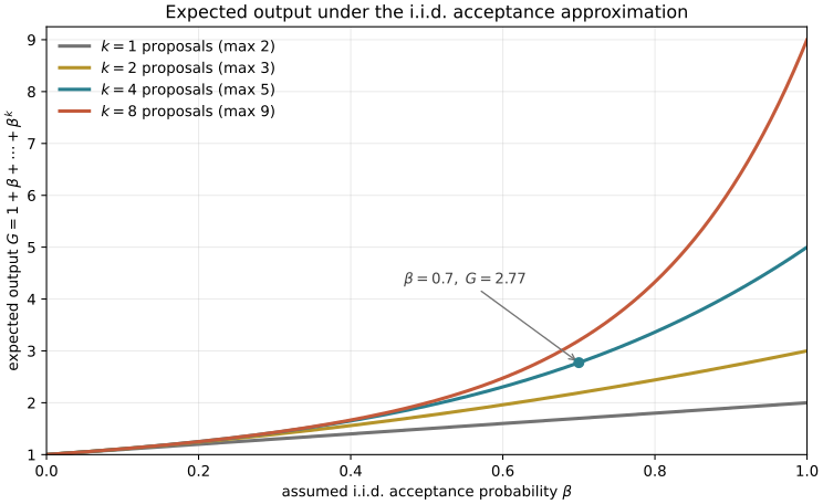
Expected output under the independent, constant-acceptance approximation. The exact expression is because acceptance varies across positions and contexts.
Speedup#
Higher number of tokens per decode is not itself the full systems speedup, other latencies need to be taken into account. Say is the latency on one decode step on target model, is the verification latency, the latency of producing all drafts and the expected number of useful output tokens. For speedup its easy to say time to produce useful draft token should be less than the decode step. Based on the system there might be another for scheduling the drafting or verification operations, for sake of this model, lets assume its very small.
Analyze this a little deeper and setup the consequent dependencies of each time term.
| Batch Size | |
| # of target model parameters | |
| Number of bytes per weight | |
| Peak FLOP/s of the accelerator | |
| Memory Bandwidth of the accelerator | |
| Target-equivalent positions evaluated during verification () | |
| Context length | |
| Existing KV-cache bytes read per sequence per decode step | |
| Existing-prefix bytes read per sequence per verification pass. | |
| Compute FLOPs per token | |
| Latency of one target decode step | |
| Latency for target verification over k proposals | |
| Latency of producing the draft |
Think of a simplified roofline model on a single device and assuming perfect memory / compute overlap. Now lets build out the and values
The critical batch size where decode becomes compute bound is when
is a constant and substituing
Similarly for , same weight traffi but times more compute is done to verify the drafts
and consequently its easy to derive that the critical batch is
For short context the KV cache traffics and which means.
This means verification becomes compute-bound much earlier than ordinary decoding, confirming that block verification has higher arithmetic intensity. But is only where verification becomes compute-bound; this is not the break-even point where speculative decoding becomes helpful. Using from above, speedup for short contexts can be defined as
Here and therefore can generally depend on batch size. Generaly, will increase with . Under this approximation, you might see three regimes coming out of this.
| Regime | Batch | Decode | Verification | Speedup |
|---|---|---|---|---|
| I | Memory-Bound | Memory-Bound | ||
| II | Memory-Bound | Compute-Bound | ||
| III | Compute-Bound | Compute-Bound |
Regime I can be flat to slightly decreasing since depending on the drafing mechanism might not change much. At fixed acceptance, regime II loses speedup as verification becomes more expensive, provided draft latency does not decrease. In regime III, the trend depends on drafting’s cost relative to ordinary decoding.
Absolute throughput can increase with batch size while the relative speedup of speculative decoding decreases. Liu et al. observe this distinction in their vLLM evaluation: for Llama 3.1 8B on GSM8K, EAGLE’s speedup drops from at batch 1 to at batch 128.12 Speculation still helps at both endpoints.
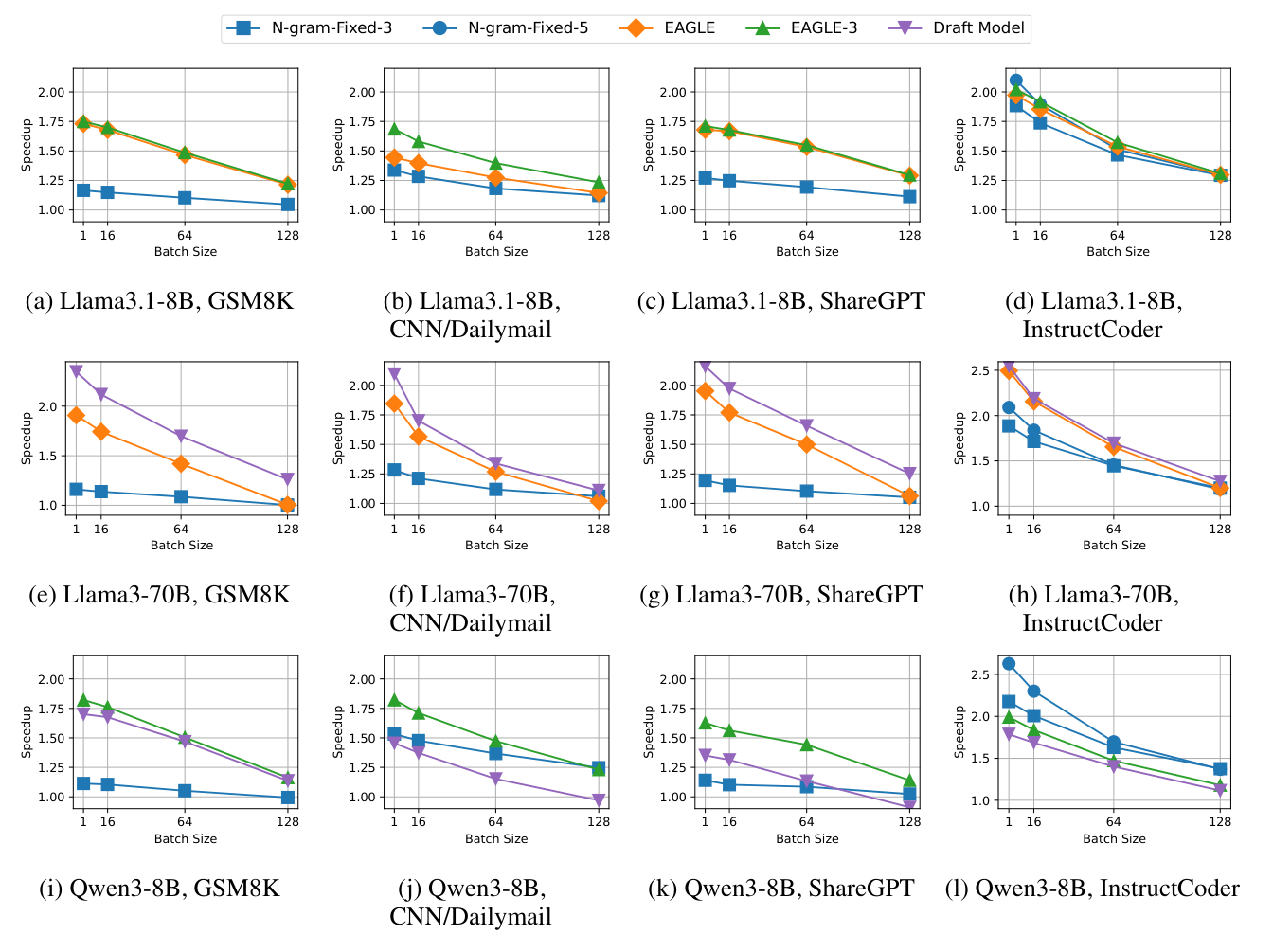
Original Figure 1 from Liu et al., Speculative Decoding: Performance or Illusion? Relative throughput versus the no-speculation baseline in vLLM, using one H100 for the 8B models and four H100s for 70B. These are workload-dependent measurements, not a controlled negligible-KV experiment or a calibration of the roofline above. Original figure cropped from the paper, reproduced under CC BY 4.0.
Long-Context effects#
While short-context gives a decreasing trend; for medium-to-long context length there is a transition towards a memory bound regime again because while the weight loading can be amortized over a batch, KV cache needs to be loaded for each request.
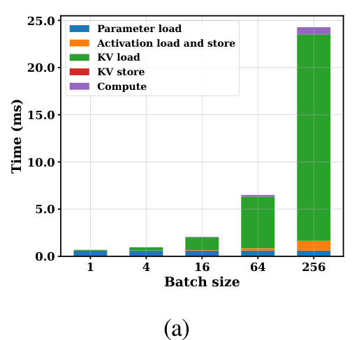
Original Figure 1(a) from Sadhukhan et al., MagicDec: Llama 3.1 8B, 16,384 input tokens, eight H100 GPUs. The breakdown shows target decoding costs, not speculative speedup. Original panel cropped from the paper, reproduced under CC BY 4.0.
This creates another interesting relation. can also be written as
If existing KV reads dominate both decode and verification latency, and both achieve comparable memory bandwidth, this is true
Verifcaiton and target decode do share a prefix so the ratio depends on how well does our inference engine support this KV reuse. At one end where there is no KV reuse the penalty is paid in speedup. At the other end where , KV values are loaded once and resuse for all proposals. Reality is often somewhere between these. Assuming the best KV resuse is about constant in the long context regime.
With fixed now speedup mainly depends on ratio only, where grows with the context length and batch, but is highly dependeny on the proposal mechanism. falls when draft latency grows more slowly as compared to the target latency and can flatten when both scale with B.
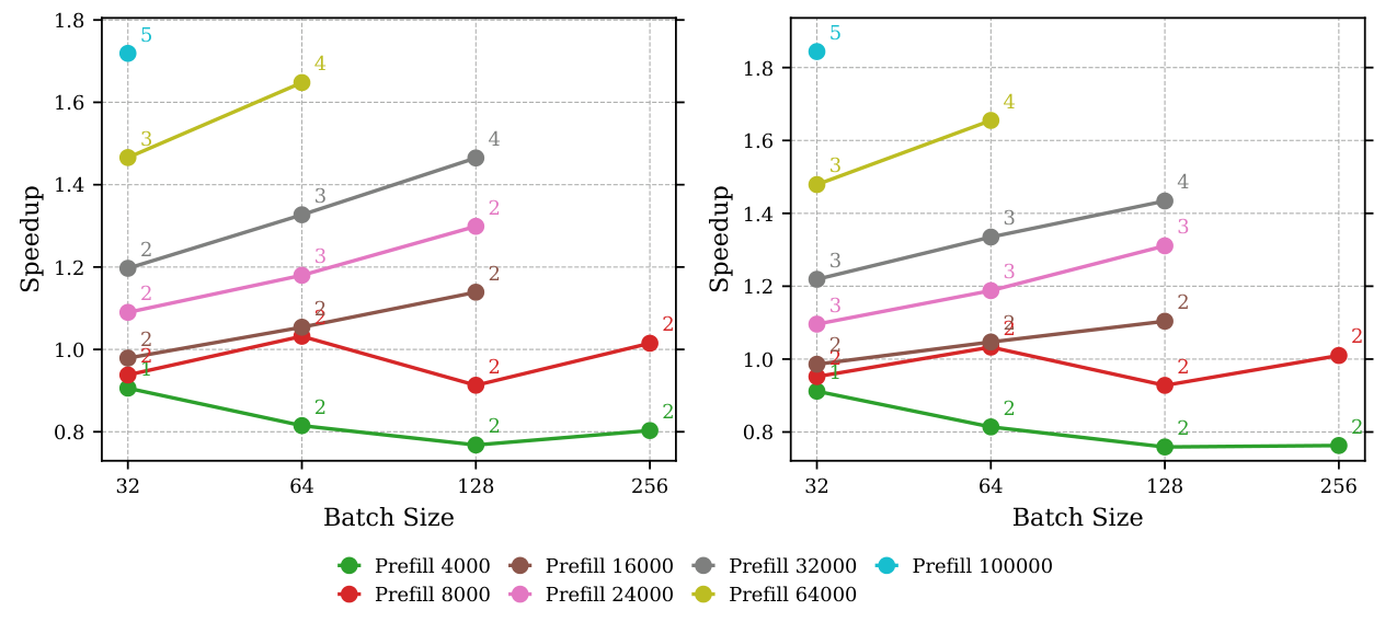
Original Figure 6 from Sadhukhan et al., MagicDec: StreamingLLM-based self-speculation with Llama 3.1 8B on PG-19, eight A100 GPUs and eight-way tensor parallelism. Draft KV budgets are 256 tokens (left) and 512 (right). Each point uses its optimal speculation length, annotated beside it. Original figure cropped from the paper, reproduced under CC BY 4.0.
Choosing drafting width#
Another interesting question to ask is: What is the optimal ? A wider draft exposes more parallel target work, but later proposals are useful only when every proposal before them survives. At the same time, both drafting and verification generally become more expensive. Intuition would say that small width is bad since you are not doing enough work, while large is also bad since saturates very quickly. There should be a middle ground. Simply, the optimal would be
Let . Adding one more speculative position is useful while
At the crossover the two sides are equal. This isn’t easy to solve analytically, but there are insights that can be extracted from it. Since ,
and therefore
This means the benefit of adding new tokens drops exponentially (). On the other hand, is expected to increase as grows, with eventually growing linearly once verification becomes compute-bound and depending on the proposal mechanism.
The optimal width is controlled by both an algorithmic limit, where prefix-survival probability becomes too small, and a hardware limit, where verification consumes the remaining compute capacity. In practice the algorithmic limit usually arrives first, which is why useful draft widths remain in the single digits even when an ideal roofline suggests capacity for hundreds of positions13. This also suggests that should not necessarily be fixed. A serving system can draft farther when the proposer is confident and stop early when the estimated survival probability of the next token no longer repays its marginal cost.14
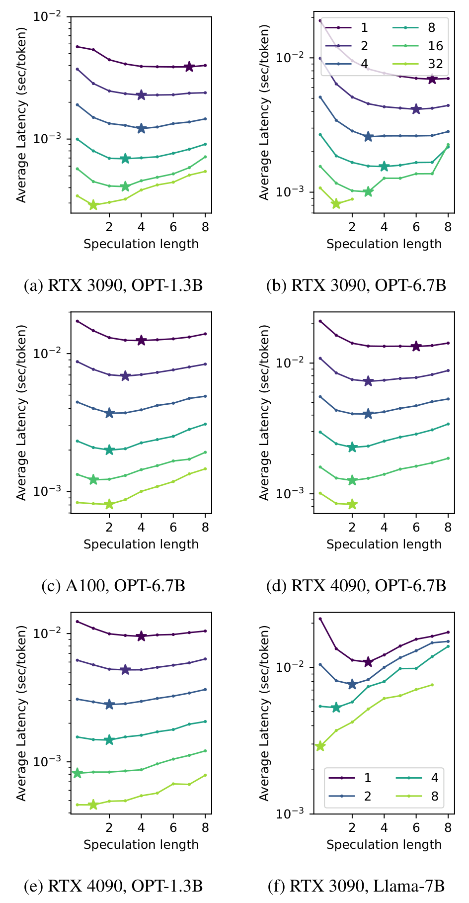
Original Figure 1 from Su et al., The Synergy of Speculative Decoding and Batching. Curves denote batch sizes; stars mark the best tested speculation length. The horizontal axis counts proposed tokens (our , so ), and the vertical axes show latency on logarithmic scales. Original figure cropped from the paper, reproduced under CC BY 4.0.
Optimization Design Space#
Lets sum up the design space that follows directly from the speedup equation:
- : better drafts.
- : faster proposal mechanisms, n-grams, prompt lookups, retrieval, etc.
- : adaptive , trees, and dynamic speculation that increase useful output per unit of verification time.15
- at fixed : better block kernels and KV reuse.
- Specialize the drafting and verification stages: disaggregated drafting.
Trees and wider candidate sets can increase both and , so is the relevant verifier-efficiency ratio rather than alone. End to end, the objective is still .
The last axis can even become a hardware topology. NVIDIA describes an external-drafter configuration where Groq 3 LPX runs the draft model and Vera Rubin NVL72 verifies and commits tokens.16 Each rack maintains its own model’s KV cache. Draft tokens are sent to the verifier, which returns rejected-position feedback for the next chunk. This is the same algorithmic decomposition expressed physically: one system manufactures future tokens and another verifies them.
I think this should be enough of an introduction to speculative decoding to convince you that it is not just some weird trick that came out of non-obvious concepts. It is a systems technique for converting predictable future work into concurrency while preserving the original decoder distribution.
Footnotes#
-
The two foundational works are Leviathan et. al., Fast Inference from Transformers via Speculative Decoding and Chen et al., Accelerating Large Language Model Decoding with Speculative Sampling. They independently report roughly latency improvements while preserving the target distribution. ↩
-
At low token batches, autoregressive decoding is commonly dominated by parameter and KV-cache movement rather than arithmetic. See Pope et al., Efficiently Scaling Transformer Inference and Chen et al., Accelerating Large Language Model Decoding with Speculative Sampling. ↩
-
You can actually say that you would change the model architecture to do parallel decode, in turn increasing the arithmetic intensity of the decode operation. This would also, theorectially, be a new axis to look at. ↩
-
See Shazeer, Fast Transformer Decoding: One Write-Head is All You Need for multi-query attention, vLLM for PagedAttention, and SGLang for RadixAttention. ↩
-
You might still be bound by KV-cache bytes per token since they must be loaded separately for each request in the batch. ↩
-
Shannon’s Prediction and Entropy of Printed English is the classic information-theoretic study of redundancy and predictability in natural language. ↩
-
For this first intuition, both the proposer and target use greedy decoding. ↩
-
Stern, Shazeer, and Uszkoreit, Blockwise Parallel Decoding for Deep Autoregressive Models developed this idea for greedy decoding before lossless speculative sampling generalized it to stochastic decoding. ↩
-
Temperature, top-k, and top-p can all be viewed as transformations that produce the final distribution from which a token is sampled. ↩
-
This resembles rejection sampling, but standard rejection sampling uses a global envelope and repeatedly samples from , accepting with probability . Speculative sampling instead accepts the maximal shared mass and, on rejection, samples once from the residual target mass . This is why Chen et al. call it modified rejection sampling. ↩
-
Wiki Total Variational Distance. ↩
-
Liu et al., Speculative Decoding: Performance or Illusion?, Section 3.2 and Figure 1. Speedup is measured as the ratio of generated-token throughput with and without speculative decoding. See Tables 5 and 6 for hardware and proposal configurations. ↩
-
At , an ideal H100 BF16 roofline gives FLOP/byte and, for short context with and , . This is a theoretical hardware ridge, not a useful draft width. ↩
-
Dynamic Speculation Lookahead Accelerates Speculative Decoding of Large Language Models shows that a fixed lookahead is generally suboptimal and reports improvements from selecting it dynamically. ↩
-
Tree verification explores several candidate futures instead of one chain. See SpecInfer and Sequoia. ↩
-
NVIDIA, How NVIDIA Groq 3 LPX Unlocks Ultrafast Interactivity at Long Context on NVIDIA Vera Rubin. NVIDIA calls this configuration external-drafter speculative decoding. ↩