Hierarchical Navigable Small Worlds
A deep dive into HNSW, an approximate nearest neighbor search algorithm.
You might have heard of this algorithm during the RAG-mania of late. But not many sources on the web go into the inner workings and intuition building, which I would like to cover here.
Hierarchical Navigable Small Worlds (HNSW) is a top-performing and popular approximate nearest neighbor search algorithm. To find the exact nearest neighbor given a bunch of vectors, we need to find a vector that is the closest to a query vector. i.e. given a set of vectors , and a query , distance function the goal is
The trivial but brute force way to do this is just iterate through all the vectors, find a minimum by distance. This is not scalable since the amount of vectors can be in billions. Another aspect of this is the number of vector dimensions which can be as large as 4096 in latest state of the art embedding models. We would also want to eliminate any extra distance calculations, since the time spent in these will not be small.
Delaunay Triangulation#
A common approach when wanting to optimize for multiple queries, is to look for a data structure we can build on top of current data so we can spend some compute and memory to lower the per query cost exponentially. What if we could store a “region” around every vector, such that all points in that region are the closest to the vector. A query point if it falls into ‘s region, by definition is the nearest neighbor of .
These regions are called Voronoi Cells and if we draw the region boundaries, this becomes a Voronoi Diagram. Here is a small visualization.

We can also represent each point as a node in a graph, and each adjacent cell as neighbors to the node. This is a mathematically equivalent representation of the Voronoi Diagram and is called Delaunay triangulation. This way for each point in the graph, finding the nearest neighbor is trivial, we just need to get the nearest out of the neighbors of the current node.

Delaunay triangulation graph where nodes represent points and edges connect adjacent Voronoi cells
But our problem statement is for point outside the given set of points, how do we use the Delaunay triangulation to answer this question? Imagine we are at a point , such that the point is not in the Voronoi cell of . What is a good decision I can make given the local information I have about my neighbors? I can find a neighbor such that . But will this work? Let’s say we move to and repeat this process. We can see that we strictly decrease the until we reach a point where we can find no such such that , which means is the nearest neighbor of .

Delaunay Walk: starting from an arbitrary point, we greedily move to closer neighbors until reaching the nearest neighbor of q
You might have noticed that we selected any closer neighbor and not the closest neighbor in the Delaunay Walk, since the process converges to produce the correct answer anyways, picking the closest adds extra computation for a reduction in number of steps the algorithm takes to converge.
The big problem with this is the curse of dimensionality, the amount of space needed to store the graph grows superpolynomially1 and becomes infeasible to store beyond small dimensions. This can be easily skirted if we consider an approximate problem, we can cap the number of neighbors to in which case, the memory requirements reduce to . But we lose the monotonic routing behavior we discussed earlier.
Small Worlds and their Navigation#
You might have heard about the six degrees of separation experiment in which social psychologist Stanley Milgram2 asked people to send a letter to a target individual, but a person can only forward the letter to a single acquaintance that they know on a first name basis. About a third of the letters reached the target person with a median of 6 steps. These and similar experiments serve as the basic evidence of existence of short paths in the global friendship network, linking all (or almost all) of us together in society.
This kind of small world phenomena is also present in a lot of places outside society, e.g. the internet itself, power grids, the fully mapped biological neural network of the worm C. elegans and many more. All this happens because of “long-range links” between local clusters, e.g. most of your friends are local; the one overseas friend can shorten the total number of links needed to reach the destination.
The same concept can work if we add these long range links to the Delaunay graph. We can randomly add new links but adding too many of them, we lose local structure and the greedy walk will not easily converge since we can’t determine if we are moving closer or not, we need to settle on some middle ground strategy. The optimal result comes from Jon Kleinberg3. Kleinberg analyzed a lattice in d dimensions, where long range links are added with the probability of link from , based on the distance between them.
- If is low; the distance doesn’t matter much. Long links are just as likely as short ones. Jumps can overshoot the target.
- If is high; the penalty of distance is huge. We mostly just link to nearby links. Jumps can be too timid and might not help.
Kleinberg proved that the optimal result occurs at .

NSW graph: local edges provide structure while long-range links (dashed) enable faster traversal across the graph
Intuition Behind and Runtime Cost#
The number of points at distance in a -dimensional space grows . And the probability of linking to one such node is . This means the total probability of reaching distance is . Now at , this probability becomes constant, i.e. we can reach any distance with the same probability and creates a Scale Invariance in the graph.
Due to the Scale Invariance property of the long-range links, we can imagine a “ring” between distance to . There would be such rings. The probability of finding a link to a certain link in a ring is constant. Let’s try to calculate this. We know , but we need to normalize the probability. The normalization denominator would be.
substituting the ring distances we get
at , this becomes a sum of s.
this implies the probability of reaching a ring is, ring’s weight () divided by .
Our goal to move to the Ring from a previous ring , we have only two choices either we find a long-link and move or continue to explore in the current ring. The expected number of trials before we succeed is , 4 this implies expected number of steps to exit the ring is . Hence.

Expected steps vs α in 2D: the sweet spot is at α = d = 2 where scale invariance emerges
This is a good improvement, but the algorithm still is very sensitive to input data and has a tendency to get stuck in a local minimum when data is highly clustered. This means expensive restarts or adding more links, both of which increase runtime, we have to tradeoff latency to get a better recall. HNSW tries to fix robustness while providing an query time.
Hierarchical Navigable Small Worlds5#
The NSW greedy walk’s run can be seen as a set of zoom in and zoom out phases. Zoom in phase goes to nodes that are highly clustered, on the other hand the zoom out phases travels long distances. Zoom in phases can get stuck in local minimas, forcing us to do costly restarts.
What if we separate out links of different length; start from the longest ones and progressively switch to shorter ones as we exhaust possibilities in the longer ones. This could add some robustness since we are not constantly zooming in and out. Another benefit of this approach is that the number of links will be a lot less in initial steps and we can explore a larger part of the graph, making our search cheaper.
This is the key idea behind the Hierarchy of HNSW, we create layers of graphs each with increasing coarseness, akin to having different zoom levels.
- Layer 0: All the nodes, edges are short and local.
- Layer 1: Fewer nodes, medium length edges.
- …
- Layer L: Top level; very few nodes, we can globally traverse the graph in handful of hops.
This is structurally very similar to Skip Lists.6 7
Querying this structure is easy; we can start on the top layer; just do the same greedy walk on each layer and move to next layer when we exhaust our options.
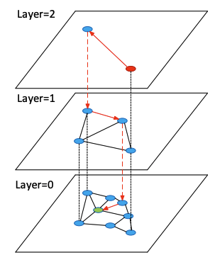
HNSW search traversal: starting from the top sparse layer, greedily descending through progressively denser layers.8
Construction#
Let’s talk construction, so when adding a node to layer , we need to (a) add it to all the layers below down to . How do we find a layer for a new node? Also, what would be the best distribution of nodes across layers for fast queries. We can take a similar geometric distribution from previous section, since we will get exponentially decreasing nodes in each layer and about layers. So , 9 here the tunable parameter. Note that this is constant per layer and not dependent on the number of nodes. This means
To find , we sum all the probabilities.
Using sum of the geometric series, for .
So
We can also compute the tail probability .
Factoring out
When sampling the level , from uniform random distribution we see.
It is also interesting to observe the the expected number of nodes in a layer will be
and the ratio of the layer sizes is
Therefore, can also be thought of as a zoom factor.
Neighbor Selection Heuristic#
While adding a node we also have to select neighbors to add, we can use the
naive strategy of just picking the nodes closest to us, but this strategy
has the same issues with robustness as previously discussed. But we can easily
add link diversity using a simple heuristic. We add a neighbor iff the neighbor
is closer to us than any other neighbors, otherwise we skip. This strategy
creates room in the node cap for longer links to fill. To implement this we
can Sort candidates by distance to the new node; keep a candidate if it is not
too close to any already selected neighbor dist(candidate, selected) < dist(candidate, new).
Intuition Behind Runtime Cost#
What is the runtime cost then? We know that we have layers; we just need to find the amount of work needed per layer. Imagine we have just come down from layer to . Search on this layer would always terminate before encountering a node that is also present in , otherwise the new point in would have been the entrypoint to layer . The probability of a point being present in both and is
Note that this is independent of layers and number of nodes. While on a walk of layer we say is probability of finding the point in (from above). The probability of continuous successes is . The expected number of steps using similar logic as NSW follows as , since , we get . This is independent of number of nodes hence the total search complexity is .
Implementation#
I am implementing this in Zig, all nodes are stored as indices of a global
vector array. Here is the definition of a Node. You might have noticed that
we have different sizes for neighbors in layer 0. In practice if we add more
neighbors in layer 0 it can improve the recall. We generally set
neighbor_size0 = 2*neighbor_size. Each node has neighbors in multiple layers.
pub const NodeIdx = u32;

const Node = struct {
    neighbors: []std.ArrayListUnmanaged(NodeIdx),

    pub fn initEmpty(
        alloc: std.mem.Allocator,
        layer: usize,
        neighbor_size: usize,
        neighbor_size0: usize,
    ) !Node {
        const neighbors = try alloc.alloc(std.ArrayListUnmanaged(NodeIdx), layer + 1);
        for (neighbors, 0..layer + 1) |*nbrs, l| {
            nbrs.* = .empty;
            const node_cap = if (l == 0) neighbor_size0 else neighbor_size;
            try nbrs.ensureTotalCapacityPrecise(alloc, node_cap);
        }

        return .{ .neighbors = neighbors };
    }
};
Now we define the main data structure for HNSW, here Params as tunable parameters for the algorithm.
max_neighbors_per_layer: () Max. number of neighbors of a node. Large values can increase recall but at the cost of runtime.ef_construction: Construction entry factor, number of nearest candidates kept during construction.ef_search: Search entry factor, number of nearest candidates kept during search.layer_mult: () Layer Multiplier, usually set to approx.max_neighbors_per_layer.
pub const HnswIndex = struct {
    pub const Params = struct {
        max_neighbors_per_layer: usize,
        ef_construction: usize,
        ef_search: usize,
        num_words: usize,
        layer_mult: f64,
        seed: u64 = 2026,
    };

    // ...omitted boilerplate vars...

    entry_points: std.ArrayListUnmanaged(NodeIdx),
    layers: usize = 0,
    nodes: std.ArrayListUnmanaged(Node),
    visited: std.DynamicBitSetUnmanaged,
}
Let’s add the function to search a single layer. We maintain two heaps: one to
store the node candidates we want to consider, and farthest which keeps the
current best ef results (its top is the worst among them). The rest is
standard best first search.
fn searchLayer(
    self: *HnswIndex,
    layer: usize,
    idx: NodeIdx,
    entry_points: std.ArrayListUnmanaged(NodeIdx),
    entry_factor: usize,
) !std.ArrayListUnmanaged(NodeIdx) {
    self.visited.unsetAll();

    var candidates = std.PriorityQueue(SearchEntry, void,minCompareSearch).init(self.allocator,{});
    defer candidates.deinit();
    var farthest = std.PriorityQueue(SearchEntry, void, maxCompareSearch).init(self.allocator, {});
    defer farthest.deinit();

    for (entry_points.items) |entry_point| {
        self.visited.set(entry_point);
        try candidates.add(.{ .idx = entry_point, .dist = self.dist(idx, entry_point) });
        try farthest.add(.{ .idx = entry_point, .dist = self.dist(idx, entry_point) });
    }

    while (candidates.count() > 0) {
        const curr_candidate = candidates.remove();
        const curr_idx = curr_candidate.idx;
        const curr_distq = curr_candidate.dist;
        const curr_farthest = farthest.peek();

        if (curr_distq > curr_farthest.?.dist) {
            break;
        }

        for (self.nodes.items[curr_idx].neighbors[layer].items) |nbr| {
            if (!self.visited.isSet(nbr)) {
                self.visited.set(nbr);
                const nbr_dist = self.dist(nbr, idx);
                const curr_farthest_ = farthest.peek();
                if (farthest.count() < entry_factor or nbr_dist < curr_farthest_.?.dist) {
                    try candidates.add(.{ .idx = nbr, .dist = nbr_dist });
                    try farthest.add(.{ .idx = nbr, .dist = nbr_dist });
                    if (farthest.count() > entry_factor) {
                        _ = farthest.remove();
                    }
                }
            }
        }
    }

    const count = farthest.count();
    var results: std.ArrayListUnmanaged(NodeIdx) = .empty;
    try results.resize(self.allocator, count);
    var i: usize = count;
    while (farthest.count() > 0) {
        i -= 1;
        const entry = farthest.remove();
        results.items[i] = entry.idx;
    }

    return results;
}
For insertion, we assign a random layer using the sampling method discussed
earlier. Then search for entry_points into the assigned_layer, with
entry_factor = 1. Then add the new node from the assigned_layer down to
0.
pub fn insert(self: *HnswIndex, idx: NodeIdx) !void {
const random = self.prng.random();
const urandom = random.float(f64);
const assigned_layer: usize = @intFromFloat(std.math.floor(
-std.math.log(f64, std.math.e, urandom) / std.math.log(f64, std.math.e, self.layer_mult),
));
const node = try Node.initEmpty(
self.allocator,
assigned_layer,
self.params.max_neighbors_per_layer,
self.max_neighbors_layer0,
);
try self.nodes.append(self.allocator, node);
if (self.nodes.items.len == 1) {
try self.entry_points.append(self.allocator, idx);
self.layers = assigned_layer;
return;
}
if (assigned_layer == self.layers) {
try self.entry_points.append(self.allocator, idx);
}
var curr_entry_points: std.ArrayListUnmanaged(NodeIdx) = self.entry_points;
var current_layer = self.layers;
var current_nearest: std.ArrayListUnmanaged(NodeIdx) = undefined;
while (current_layer > assigned_layer) {
const new_entry_points = try self.searchLayer(current_layer, idx, curr_entry_points, 1);
curr_entry_points = new_entry_points;
current_layer -= 1;
}
current_layer = @min(assigned_layer, self.layers) + 1;
while (current_layer > 0) {
current_layer -= 1;
current_nearest = try self.searchLayer(
current_layer,
idx,
curr_entry_points,
self.params.ef_construction,
);
try self.selectNeighbors(current_layer, idx, ¤t_nearest);
for (current_nearest.items) |nbr_idx| {
try self.nodes.items[idx].neighbors[current_layer].append(self.allocator, nbr_idx);
const nbr_neighbors = &self.nodes.items[nbr_idx].neighbors[current_layer];
try nbr_neighbors.append(self.allocator, idx);
const max_neighbors = if (current_layer == 0) {
self.max_neighbors_layer0
} else {
self.params.max_neighbors_layer0
};
if (nbr_neighbors.items.len > max_neighbors) {
try self.selectNeighbors(current_layer, nbr_idx, nbr_neighbors);
}
}
curr_entry_points = current_nearest;
}
if (assigned_layer > self.layers) {
self.layers = assigned_layer;
self.entry_points.clearRetainingCapacity();
try self.entry_points.append(self.allocator, idx);
}
}Now we add the selectNeighbors function, this is the neighbor selection
heuristic discussed earlier. We can sort the neighbors and skip nodes that are
closer to another neighbor than to the query idx.
fn selectNeighbors(
    self: *HnswIndex,
    layer: usize,
    idx: NodeIdx,
    candidates: *std.ArrayListUnmanaged(NodeIdx),
) !void {
    const max_neighbors = if (layer == 0) {
        self.max_neighbors_layer0
    } else {
        self.params.max_neighbors_per_layer
    };

    var candidate_entries: std.ArrayListUnmanaged(SearchEntry) = .empty;
    defer candidate_entries.deinit(self.allocator);

    for (candidates.items) |c| {
        try candidate_entries.append(self.allocator, .{ .idx = c, .dist = self.dist(c, idx) });
    }

    candidates.clearRetainingCapacity();

    std.mem.sort(SearchEntry, candidate_entries.items, {}, minCompare);

    for (candidate_entries.items) |c| {
        var good = true;
        for (candidates.items) |s| {
            if (self.dist(c.idx, s) < c.dist) {
                good = false;
                break;
            }
        }
        if (good) {
            try candidates.append(self.allocator, c.idx);
        }
        if (candidates.items.len >= max_neighbors) {
            break;
        }
    }
}
Lastly we can add topK to find the K nearest neighbors. Here we just greedily
search nodes in all layers except layer 0. On layer 0, we cast a larger net and
filter out the top k nodes.
pub fn topK(self: *HnswIndex, idx: NodeIdx, k: usize) !std.ArrayListUnmanaged(NodeIdx) {
    var candidates: std.ArrayListUnmanaged(NodeIdx) = undefined;
    var curr_entry_points = self.entry_points;
    var curr_layer = self.layers;

    while (curr_layer > 0) {
        const new_entry_points = try self.searchLayer(curr_layer, idx, curr_entry_points, 1);
        curr_entry_points = new_entry_points;
        curr_layer -= 1;
    }

    candidates = try self.searchLayer(0, idx, curr_entry_points, self.params.ef_search);
    candidates.shrinkRetainingCapacity(k);
    return candidates;
}
This implementation is not going to be very performant, since I am not using a lot of optimal data structures and we have a lot of pointer chasing. On my AMD Ryzen 9 9950x3D (single core) using the GloVe Dataset’s 50-dim sample (1.29M vectors), I am getting these results.
- Index build time: 93.10s
- Average recall: 75.00%
- Average query time: 92.0µs (100 queries, k=10)
This seems good enough for a quick and dirty implementation. Code can be found on Github. Perhaps I will create another post about optimizing this in the future.
Footnotes#
-
Why? See McMullen’s Upper Bound Theorem ↩
-
Travers, Jeffrey, and Stanley Milgram. “An experimental study of the small world problem.” Sociometry (1969): 425-443. ↩
-
Kleinberg, Jon. “The small-world phenomenon: An algorithmic perspective.” Proceedings of the thirty-second annual ACM symposium on Theory of computing (2000). ↩
-
This follows from the geometric distribution. If each trial succeeds with probability , then . Intuitively: with , you expect 2 coin flips to get heads; with , you expect 10 trials. ↩
-
Malkov, Yu A., and D. A. Yashunin. “Efficient and robust approximate nearest neighbor search using Hierarchical Navigable Small World graphs.” IEEE transactions on pattern analysis and machine intelligence 42.4 (2018): 824-836. arXiv:1603.09320 ↩
-
This is not the same in the original paper. Original paper uses . But in my opinion framing leads to better intuition. ↩